Denormalizing tables in Power Query

Given a great number of Power Query data load and transform scripts will end up populating an Excel Data Model, it is important to keep in mind that a dimensional approach is preferred when shaping data.  Clearly one of the steps we want to follow, whenever possible, is that of denormalizing tables to more properly reflect logical entities.

Using the Power Query UI, it is easy enough to load tables and merge them.  Unfortunately, relying solely on the UI can generate a rather inefficient process involving multiple M scripts.

Let’s say for example that we want to combine Adventure Works tables DimProduct, DimProductSubcategory and DimProductCategory to create a consolidated Product table containing a few product attributes as well as the subcategory and category names.

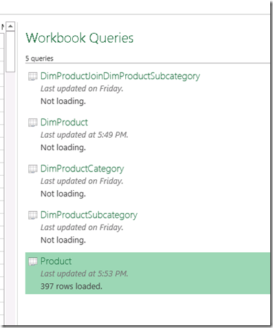
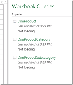
If you start querying table by table, you end up with three workbook queries.  As we are not yet ready for loading into the Data Model, I have unselected that option.

image

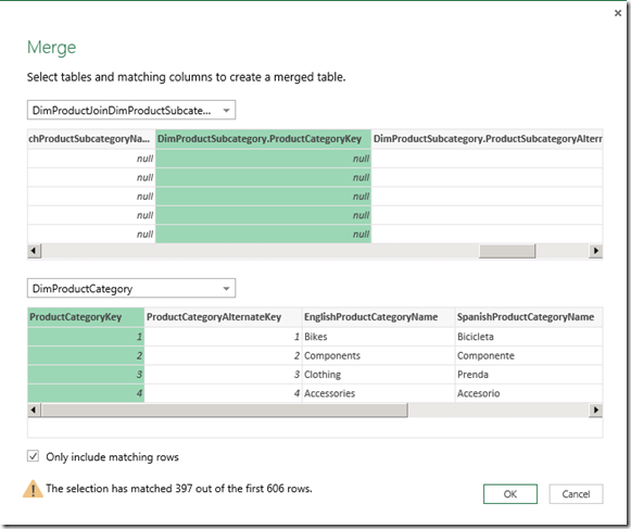
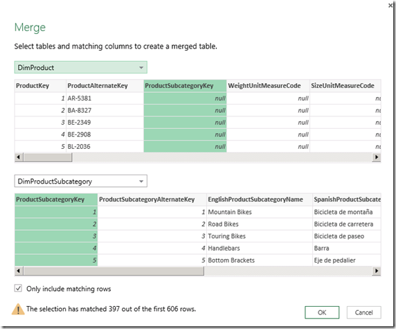
We still need two additional scripts to denormalize.  One will consolidate DimProduct into DimProductSubcategory (we can call the ouptut DimProductJoinDimProductSubcategory).  By selecting the Merge option in the toolbar, we are presented with a window that allows us to merge two resultsets by specifying a matching column.  In this case, we start by merging DimProduct with DimProductSubcategory via the ProductSubcategoryKey.

image

Unfortunately, as this window only allows us to merge two datasets at once, we have to walk one more step in order to merge DimProductJoinDimProductSubcategory with DimProductCategory and get all the necessary data we want in one table.  

image

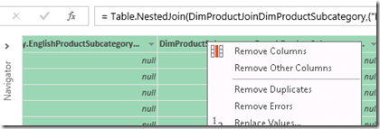
As the result of this process will contain columns from all tables, we must remove the columns we don’t need.

image 

Finally we end up with the table we were looking for: “Product”:

image

Though it was fairly easy to do, its a relatively inefficient process that requires the refreshing of 4 intermediary scripts that add little to no value as independent queries:

image

Instead, we are better off generating the denormalizing effect as a single M script, which actually runs more efficiently as:

  • requires one query refresh instead of five.
  • selects only the required columns (improving efficiency), instead of selecting all columns and then removing the unwanted ones.

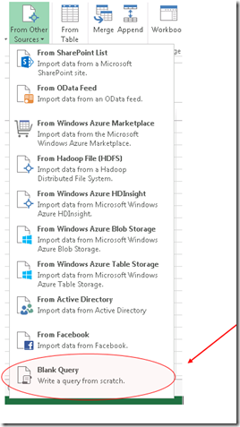
To do so, we can start instead with a blank query,

image

and on it, replicate the steps followed before but this time using systematic, step by step approach that consolidates all steps and does not require maintenance of separate scripts:

let
    Source = Sql.Database("localhost", "AdventureWorksDW2012"),
    DimProduct = Source{[Name="DimProduct"]}[Data],
    DimProduct.Result = Table.SelectColumns (DimProduct,
                {"ProductKey",
                "EnglishProductName",
                "Color",
                "ModelName",
                "ProductSubcategoryKey" } ),

    DimProductSubcategory = Source{[Name="DimProductSubcategory"]}[Data],
    DimProductSubcategory.Result = Table.SelectColumns ( DimProductSubcategory,
                {"EnglishProductSubcategoryName",
                "ProductSubcategoryKey",
                "ProductCategoryKey"}),

    DimProductCategory = Source{[Name="DimProductCategory"]}[Data],
    DimProductCategory.Result = Table.SelectColumns ( DimProductCategory,
                {"EnglishProductCategoryName",
                "ProductCategoryKey"}),

    /* Join DimProduct to DimProductSubcategory */
    DimProductJoinDimProductSubcategory = Table.Join(DimProduct.Result,
               "ProductSubcategoryKey", DimProductSubcategory.Result , "ProductSubcategoryKey" ) ,  

    /* Join Product and Subcategories to Categories */
    Product = Table.Join( DimProductJoinDimProductSubcategory, "ProductCategoryKey",
               DimProductCategory.Result, "ProductCategoryKey" ),

    /* Select Final Result */
    Product.Result = Table.SelectColumns (Product, {
        "ProductKey",
        "EnglishProductName",
        "EnglishProductSubcategoryName",
        "EnglishProductCategoryName",
        "Color",
        "ModelName" } )  

in
    Product.Result


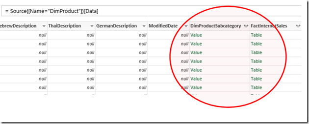
The result is highly efficient and more easily maintained.  Another way in which this process can be done, if there are existing relationships among tables, is by the process of ‘expanding columns’. These are columns that are automatically loaded and represent a link to another table that has a relationship with the table we are loading. You can see them in the UI as:

image 

Following a similar approach to the one outlined before, we can device a single M script to do all the work.  This time, we will expand the columns without the need to explicitly join tables, achieving the same denormalized result:

let
    Source = Sql.Database("localhost", "AdventureWorksDW2012"),

    /* load DimProduct */
    qryProd = Source{[Name="DimProduct"]}[Data],

    /* retrieve Subcategory Name */
    qrySubCat = Table.ExpandRecordColumn(
        qryProd,
        "DimProductSubcategory",
        {"EnglishProductSubcategoryName", "DimProductCategory" }),

   /* retrieve Category Name */
    qryCat = Table.ExpandRecordColumn(
        qrySubCat,
        "DimProductCategory",
        {"EnglishProductCategoryName"}),

    /* select columns of interest */
    Product = Table.SelectColumns (qryCat , {
        "ProductKey",
        "EnglishProductName",
        "EnglishProductSubcategoryName",
        "EnglishProductCategoryName",
        "Color",
        "ModelName" } )   

in
    Product


The Table.ExpandRecordColumn function allows you to navigate pre-established relationships. Notice the first parameter is the table we are working with and the second parameter is the column we will be expanding. If we are in the ‘many’ side of the relationship, we will see a ‘Value’ string which indicates there is a single value to be returned from the lookup table.  Otherwise, we will see a ‘Table’ string.

Finally, notice that when expanding Subcategory values we not only retrieve the EnglishProductSubcategoryName (a column we want in the final resulset), but also we are retrieving a column called ‘DimProductCategory’.  This is a column with a reference to the DimProductCategory table, which is required to further expand the resultset, allowing us to jump one more step and retrieve the EnglishProductCategoryName.
Target well-formed Data Models when using Power Query

Even though Power Query gives us the ability to generate impressive data transformations, is up to the model author to define a well formed Power Pivot Data Model that respects relationship principles. In the past, I blogged about 3 options to ‘merge’ data using Power Pivot:

  • Issuing a SQL-like query to Excel data sources (here)
  • Issuing a SQL query to relational sources (here)
  • Using Excel inherent capabilities (here)
    All of the options above required applying Power Pivot data modeling principles which in essence implied the creation of two additional ‘lookup’ (dimension) tables to connect the existing fact data sets.

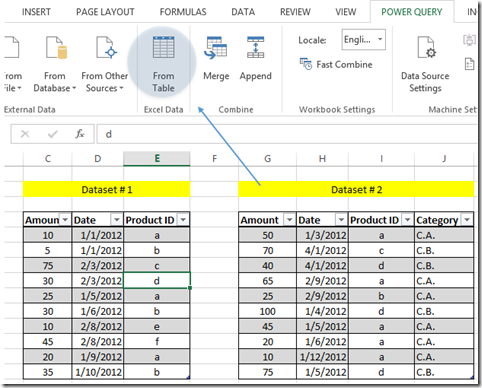
Using Power Query, the logic is similar although we use the M language.  In this blog entry, I will be also using the same small dataset which, even though its tiny, exemplifies the typical issues encountered by analysts when attempting to merge data (duplicate key records – absent lookup tables, missing values and so on).

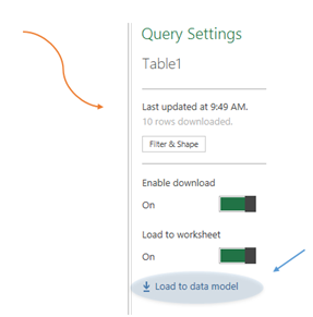
The first step is to generate 2 queries and directly load them into the model:

image

                                                                                                           image

To properly establish a relationship we must now extract two lookup tables from the data given:

  • A date lookup containing all dates across both datasets
  • a product lookup containing all products across both tables and assign an unknown value to missing categories

LOOKUP # 1 (Date Lookup)

The first one can be done with the following M query

let
    Table1Dates =
        Table.FromList(
            Table.Column(
                Table.TransformColumnTypes( Table1, { "Date", type text } ), "Date" 
                )
            ) ,
    Table2Dates =
        Table.FromList(
            Table.Column(
                Table.TransformColumnTypes( Table2, { "Date ", type text } ), "Date " 
            )
        ) ,
    CombinedTables = Table.Combine ( { Table1Dates, Table2Dates } ),
    DuplicatesRemoved = Table.Distinct( CombinedTables ),
    ChangedType = Table.TransformColumnTypes(DuplicatesRemoved,{{"Column1", type datetime}}),
    RenamedColumns = Table.RenameColumns(ChangedType,{{"Column1", "DateKey"}})
in
    RenamedColumns

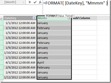
Once in the model, we can apply a DAX calculated column to extract the month name that we want to use to slice and dice:

image


LOOKUP # 2 (Product Lookup)

The second lookup table can be generated using Power Query with the following script:

let
    Source =
        Table.Join(
            Table1,{"Product ID"},
            Table.RenameColumns(
                Table2,{ "Product ID", "Product ID2"}
                ),{"Product ID2"},
            JoinKind.FullOuter
            ),
    RemovedColumns = Table.RemoveColumns(Source,{"Amount", "Date", "Amount ", "Date "}),
    DuplicatesRemoved = Table.Distinct( RemovedColumns ),
    ConsolidateProductKey = Table.AddColumn(
                                DuplicatesRemoved,
                                "ProductKey",
                                each if ([Product ID] = null) then [Product ID2] else [Product ID]
                            ),
    RemoveOriginalProductKeys = Table.RemoveColumns(ConsolidateProductKey ,{"Product ID", "Product ID2"}),
    AssignUnknownCategory = Table.AddColumn(
                                RemoveOriginalProductKeys ,
                                "Custom",
                                each if( [Category] = null ) then "Uncategorized" else [Category]
                                ),
    FinalTable = Table.RemoveColumns(AssignUnknownCategory ,{"Category"})
in
    FinalTable

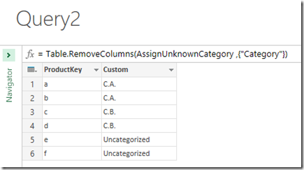
With the following result:

image

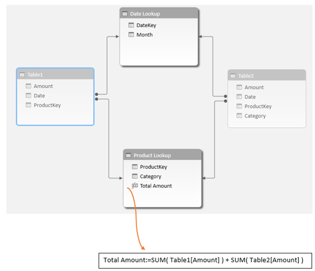
With this, we can finalize the Power Pivot Data Model using appropriate lookups and one final DAX measure:

image

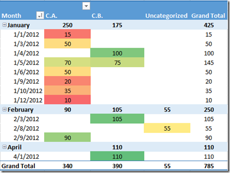
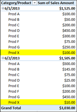
The resulting model is well-formed and can slice two tables that by themselves could not be reconciled directly in the Data Model:

image


Is this the only way?

One can argue that rather that developing a well formed data model including dimension tables it may be simpler to append one table to the other one and have the Data Model consume it as a single table.  In fact, generating a single table off the data shown is quite possible using Power Query.

However, single table data models have challenges that make their use not ideal:

  • Calculations must rely on a single base level of granularity which may not properly reflect the business model and make require workarounds and ill performing computations.
  • Given the limitation outlined above, it may be necessary to create multiple copies of the data – each targeting different granularities – with unwanted consequence of having multiple versions of the same metadata
  • Reporting tools using parameters must execute SQL DISTINCT like expressions over dimension data to remove duplicates on parameter lists, most likely affecting performance and report usability
  • Advanced modeling scenarios like many to many cannot be represented

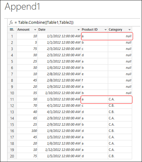
Finally, in closer examination even appending won’t do the trick in cases like the one discussed as it will fail to properly consolidate dimensions. Using the standard appending functionality, Power Query will leave, on the data used here, two designations for Product A: one with a category assigned to it, and the other one without.

image

An assumption could be that Product A *always* belongs to the same category ("C.A").  Data Analysts, as Subject Matter Experts, can confirm if such assumptions are correct.  In the example above we assumed it was, and further modeling and consolidation was needed.  The problem with the source files was that one of the columns – Category, in this case – was omitted on Dataset # 1. We ‘consolidated’ the product definitions via the M language, issuing a full outer join over the two datasets.

With this in mind, be careful on your approach to modeling of Power BI solutions.  Simplicity on Data Model development is important, but oversimplifying can harm more than help.

You can access the demo workbook here: PQ_and_data_modeling.xlsx 

Update 9/24/13: Added more details to the explanation of why appending tables should be avoided in cases like the one described.

DAX context propagation, inactive relationships and calculated columns

Marco Russo wrote recently an excellent blog post detailing the options you face when retrieving values from one table to another one via DAX’s USERELATIONSHIP function.   I found his post particularly interesting given I had written a post about a similar subject some time ago, in which a reached some conclusions that I want to revisit.

One of the solutions he describes (although he doesn’t recommend) uses the following formula signature:

CALCULATE (
    CALCULATE (
        VALUES ( <value on related column to retrieve> ), 
        <many-side table> 
    ),
    USERELATIONSHIP ( <one-side key>, <many-side key> ),
    ALL ( <one-side table> )
)

His recommended approach is instead to use LOOKUPVALUE.  However, I found the above calculation interesting and decided to break it down to understand it a bit better.   And here I ran areas of DAX that may be less than intuitive, yet worthy of a blog post.


Breaking it down

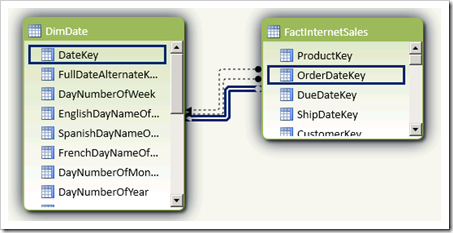
Here is the data model we use, which includes inactive relationships:

image

Step 1: To test the behavior of the inner most CALCULATE, is worth starting from a simpler starting point:

FactInternetSales[CalculatedColumn1]=
COUNTROWS( DimDate )

image

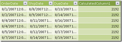
Clearly, the number reflects the total amount of records on the date table regardless of the row in context.  This in itself can be non intuitive for people starting to use DAX, as by default calculated columns evaluate under row context.  However, aggregate functions (SUM, MIN, COUNTROWS, etc) even in calculated columns will, by default, operate under filter context:  as there is no current filters in the filter context, we get the total count of rows across all date values.

Step 2: Context Transition

FactInternetSales[CalculatedColumn1]=
CALCULATE( COUNTROWS( DimDate ) )

image

Row context gets transformed into filter context and the only surviving row in the date table follows the active relationship on the data model.

Step 3: Context propagates for ALL rows in fact table at once

FactInternetSales[CalculatedColumn1]=
CALCULATE( COUNTROWS( DimDate ), FactInternetSales )

Internally, DAX generates an extended table using left outer join logic to propagate context. Given the setFilter parameter of the CALCULATE function operates on a filter context including all rows from the fact table, the resulting output is the total count of rows on the date table that have registered internet sales.  Non-intuitively, context transition does not occurs on a per row basis, even though we use CALCULATE.

image

Step 3a (test)-  Context propagates for one table, but still under active relationship:

FactInternetSales[CalculatedColumn1]=
CALCULATE( VALUES( DimDate[FullDateAlternateKey] ), FactInternetSales[ShipDateKey]  )

One may be inclined to think that using the key column of the inactive relationship as the setFilter parameter of CALCULATE will force the context propagation to retrieve the value used by the inactive relationship.  However, this is not the case and even though DAX retrieves only one value it is still the one associated with the active relationship given the internal extended table was already resolved (OrderDate)

image 

Step 3b (test)– CALCUALTETABLE returns standard context transition behavior

FactInternetSales[CalculatedColumn1]=
CALCULATE( COUNTROWS( DimDate ), CALCULATETABLE(FactInternetSales ) )

image

Wrapping CALCULATETABLE around the fact table used as setFilter parameter allows row context transition to happen again using the active relationship.

Step 4 – An outer CALCULATE propagates context using the inactive relationship, yet it collides with the current context transition using the active relationship

FactInternetSales[CalculatedColumn1]=
CALCULATE(
    CALCULATE(
        COUNTROWS( DimDate ), 
        FactInternetSales ),
    USERELATIONSHIP( DimDate[DateKey], FactInternetSales[ShipDateKey] )
)

image

If we take a peek at the DAX query plan, we understand the reason there is no output here.  Profiler trace shows 2 Vertipaq storage engine scans using different join conditions:

SELECT
[DimDate].[DateKey], […]
FROM [FactInternetSales]
    LEFT OUTER JOIN [DimDate] ON [FactInternetSales].[OrderDateKey]=[DimDate].[DateKey]

and

SELECT
[…]
FROM [FactInternetSales]
    LEFT OUTER JOIN [DimDate] ON [FactInternetSales].[ShipDateKey]=[DimDate].[DateKey]
WHERE
    ([DimDate].[DateKey], [DimDate].[FullDateAlternateKey], […]) IN {(20080421, 39559.000000, …[60398 total tuples, not all displayed]}


When the formula engine attempts to tie the results of the queries, the resulting context is empty as no date has the same shipdate and orderdate, making the two scan results incompatible.

Step 5 – Clearing the context on the active relationship key

FactInternetSales[CalculatedColumn1]=
CALCULATE(
    CALCULATE(
        COUNTROWS( DimDate ), 
        FactInternetSales ),
    USERELATIONSHIP( DimDate[DateKey], FactInternetSales[ShipDateKey] ) , ALL ( DimDate)
)


image

By the use of ALL, this time we force the query plan to remove the scan using a left outer join condition on the Order Date Key (the active relationship).  As the only other join condition that remains uses the Ship Date Key, this is the one that survives. Now we see the value returned is in fact using the inactive relationship (matching Ship Date).


Alternate Approaches for non-exact matches

As mentioned by Marco, use LOOKUPVALUE is your intent is to retrieve one value based on an exact matching condition.  In some case, though, you may want to use approximate matches – particularly when creating calculated columns as intermediate steps to measures, a common practice described on my prior post.  In this case, the approach using CALCULATE is still useful.

Two alternate solutions using a slightly more legible approach could be:

1) Using CALCULATETABLE

FactInternetSales[CalculatedColumn1]=
CALCULATE(
    VALUES(  DimDate[FullDateAlternateKey]  ),
    CALCULATETABLE( FactInternetSales,
                    USERELATIONSHIP( DimDate[DateKey], FactInternetSales[ShipDateKey] )  ,
                    ALL( DimDate ) ,
                    DimDate[CalendarYear] > 2007
                )
        )

By moving the USERELATIONSHIP to an inner CALCULATETABLE expression, it could be directly apparent we are manufacturing a table context of our own choosing and setting it as a filter parameter to the outer calculate. The third parameter of the CALCULATETABLE uses a condition not based on exact matches.

2) Using FILTER

FactInternetSales[CalculatedColumn1]=
CALCULATE(
    VALUES( DimDate[FullDateAlternateKey] ),
    FILTER(
        DimDate,
        FactInternetSales[ShipDateKey] = DimDate[DateKey] &&
        DimDate[CalendarYear] > 2007
    )
)

Interestingly, the calculation using FILTER appears to use a very efficient query plan with no extended tables generated and represented in the form Vertipaq SE scans using left outer joins. Given the setFilter parameter uses DimDate instead of FactInternetSales, there is no need to build extended tables to propagate context and the 3 scan are direct queries to tables in the data model:

SELECT
[FactInternetSales].[ShipDateKey]
FROM [FactInternetSales]

+

SELECT
[DimDate].[DateKey], [DimDate].[CalendarYear]
FROM [DimDate]

+

SELECT
[DimDate].[DateKey], [DimDate].[FullDateAlternateKey]
FROM [DimDate]
WHERE
    [DimDate].[DateKey] IN (20080105, 20080219, …[220 total values, not all displayed])

I am curious as to why the query plan did not register, on this last expression, the FILTER condition of ‘greater than’ (as it does when using the CALCULATETABLE expression).  However, due to a simpler query plan, I wonder if it could be possible the FILTER method would perform better than the CALCULATE method using USERELATIONSHIP even in cases in which only the exact match condition is needed.

Split DAX calculation steps to enhance memory utilization

An advantage of DAX measures over calculated columns is that they respond to user interaction.  As such, you may be inclined to allocate all calculation logic into measures when there is a need to respond to slicer selection, for example.

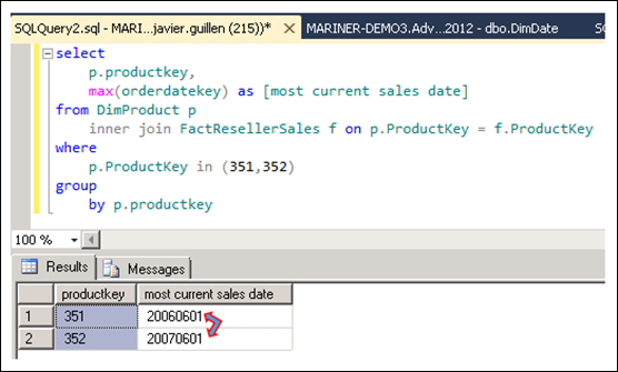
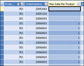
From a pure performance point of view, this may not always be optimal however.  Take the following example, in which a DAX developer intends to develop a metric for ‘most current sales amount’ per product (really, the last non empty sales amount per product).  Using Adventure Works, you can see that each product may have different  ‘last non empty dates’: 

image

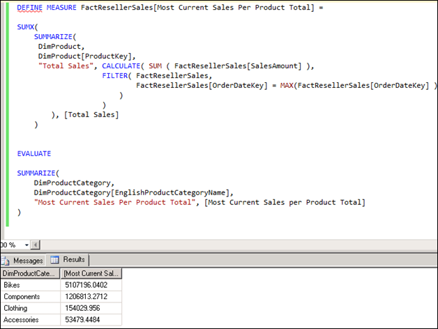
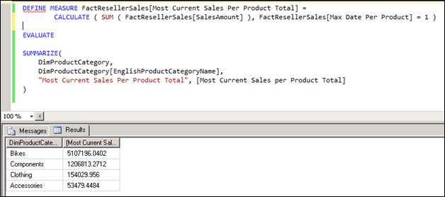
As such, a DAX measure to render the most current sales amount must first iterate on products prior to determining the sales total.  In other words, it must determine – for each product – what was the most current order date and only aggregate the sales amount on that date.  As a pure measure, this could be done as:

image

And that would give the expected result.  However, from a computation perspective it may pose efficiency problems, particularly over big fact tables and scarce RAM resources due to the iterative command inside of the CALCULATE function.

If you think about it, the most current date with sales per product is not a changing variable but instead can be predetermined.  However, the actual output could be dynamic (as the total could be filtered by user selection).  So lets break the calculation in two steps:

  • Determining most current sales date per product
  • Aggregating based on user selection

The first one can be re-allocated to a calculated column, in effect pre-computing it:

Calculate (
  CountRows ( Values ( FactResellerSales[OrderDateKey] ) ),
Filter (
  AllExcept (
        FactResellerSales,
        FactResellerSales[ProductKey],
        FactResellerSales[OrderDateKey] ),
        FactResellerSales[OrderDateKey] = Calculate (
                               Max ( FactResellerSales[OrderDateKey] ),
                               AllExcept ( FactResellerSales, FactResellerSales[ProductKey] )
                             )
               )
)

image 

leaving the second part as a measure (to allow aggregation based on user assigned filters):

image

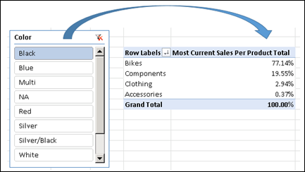
The interesting part is we are not increasing much the memory footprint of the model itself, as the resulting values on the calculated column are either 1 or blank.  However, we gain much on the way of calculation performance while still allowing for user interactive responses.  This becomes clear, for example, when calculating ratios based on the DAX measure in question:

image

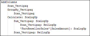
The impact in memory use is very positive, while the output accuracy remains the same.  Comparing DAX physical query plans on both methods reveals a much simpler approach which relies heavily on the Storage Engine, gaining 73% in performance:

(13 milliseconds, cold cache):

image 

In conclusion: consider pre-computing those calculation steps that do not change due to user interaction.  Doing so may allow you to more efficiently compute numbers while more efficiently manage CPU utilization.

Nurturing Model Growth: Prototyping ETL using Excel sources

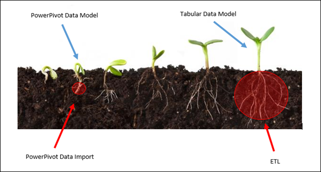
The BISM Tabular framework’s extensibility does not only imply a move from personal PowerPivot models to corporate Tabular models but also an ability to ‘branch out’ processes into more sophisticated layers of ETL and/or reporting.

Over the last months I have witnessed PowerPivot models that ‘take a life of their own’, and through their growing popularity become more sophisticated as they evolve. As their data load facilities develop further, they offer the ability to prototype ETL over a target in-memory schema, while testing assumptions regarding the appropriate data model to use.

I call these ‘seed models’ ::  that is, individual PowerPivot models that have potential for organic growth beyond its original intent – all the way into enterprise Semantic Models.  As they grow, they themselves can become the corporate standard or instead be assimilated into pre-existing Tabular models. 

image

The process of nurturing model growth (from individual to enterprise level) is a fascinating task.  This blog post explores one aspect of model expansion – from Excel files (a very common source for data analysts) to SSIS based ETL. 

It is interesting to note this expansion happens at the pace that makes most sense for the organization given its current BI maturity, and at every stage of the process there is tangible benefits to the business.

GROWTH STAGE #1:  SELF SERVICE BI BASED ON ‘DATA DUMPS’

Here you find Self-Service BI scenarios in which analysts utilize extracts from multiple systems to generate their consolidated reporting.

Assume the following datasets:

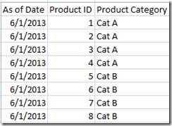
ProductList.xlsx

image


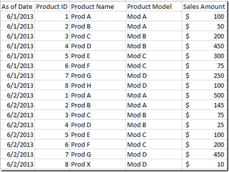
ProductSales.xlsx

image


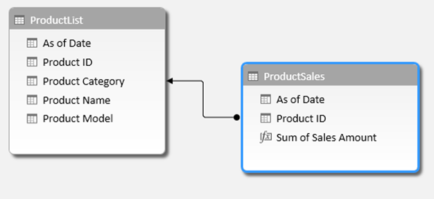
As you can see, the second workbook (ProductSales.xlsx) contains data that can be mapped back to the first one (ProductList.xlsx).  However, it is not just a fact sales table, it also contains dimension data (Product Name and Model). 

In the PowerPivot/Tabular world (just as in traditional data warehousing) it is recommended to structure data conforming logical entities. By executing a SQL query over these two Excel files it is possible to generate the necessary lookups to develop a user friendly dimensional model.

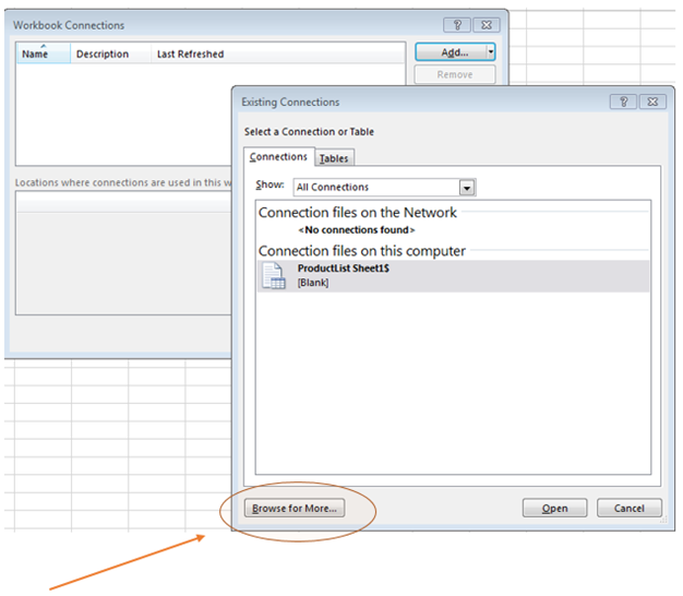
To do this, it is necessary to create a connection to the files outside of the PowerPivot window (this enables us to execute SQL queries over Excel files).

Go to Data –> Connections and click ‘Add to the Data Model’. When the next window appears, click on ‘Browse for More’

image

Find ProductList.xlsx and load it into the model.  Now follow the process again for the ProductSales.xlsx file, but this time do not add it to the data model, simply add the connection.

image

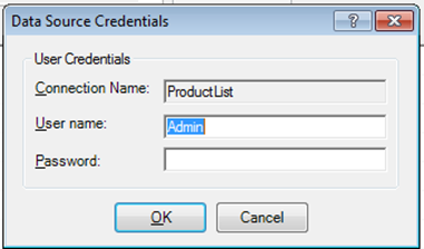
In the PowerPivot window, go to the Design tab and select ‘Table Properties’.  You will notice a prompt asking for a password, which you can simply ignore by clicking OK:

image

This prompt is not ideal as it can get on the way of automated refreshes.  To remove it, it is necessary to change the connection string,

From:

Provider=Microsoft.ACE.OLEDB.12.0;User ID=Admin;Data Source=C:\blog\ProductList.xlsx;Mode=Share Deny Write;Extended Properties="HDR=YES;";Jet OLEDB:System database=;Jet OLEDB:Registry Path=;Jet OLEDB:Engine Type=37;Jet OLEDB:Database Locking Mode=0;Jet OLEDB:Global Partial Bulk Ops=2;Jet OLEDB:Global Bulk Transactions=1;Jet OLEDB:New Database Password=;Jet OLEDB:Create System Database=False;Jet OLEDB:Encrypt Database=False;Jet OLEDB:Don’t Copy Locale on Compact=False;Jet OLEDB:Compact Without Replica Repair=False;Jet OLEDB:SFP=False;Jet OLEDB:Support Complex Data=False;Jet OLEDB:Bypass UserInfo Validation=False;Jet OLEDB:Limited DB Caching=False;Jet OLEDB:Bypass ChoiceField Validation=False


To simply:

Provider=Microsoft.ACE.OLEDB.12.0;Data Source=C:\blog\ProductList.xlsx;Extended Properties="Excel 12.0 Xml;HDR=YES"

Remember, in Excel 2013, once the connection has been modified in the PowerPivot window it is not possible to edit it (in Excel 2010 this is possible).  In other words, be sure to implement the change prior to doing any PowerPivot model work.

Warning:  Automated data refresh using Excel sources in PowerPivot for SharePoint is not currently supported (see here).  However, the refresh will work and under your discretion of ensuring controlled access to the source files it is possible to generate a solution that provides much value to the business. 

Now click on ‘Switch to Query Editor’:

image

By joining both files, we are able to mimic the type of queries we commonly use as part of ETL processes to define target dimension tables.  This process involve defining a ‘driving’ table, commonly associated with the master list of dimension attributes, which is left joined to other tables which may contain additional attributes (a common pattern in ETL development).

The SQL query to use is the following:

SELECT
[ProductList$].*,
[ProductSales$].[Product Name],
[ProductSales$].[Product Model]  
FROM ([ProductList$]
    LEFT OUTER JOIN `C:\blog\ProductSales.xlsx`.[ProductSales$] 
ON
    [ProductList$].[Product ID] = [ProductSales$].[Product ID])
WHERE
    (
    [ProductSales$].[As of Date] =
        (SELECT MAX([ProductSales$].[As of Date]) FROM `C:\blog\ProductSales.xlsx`.[ProductSales$] )
    )

The use of this query pattern gives the PowerPivot data model an important artifact: a lookup table. Generating valid lookup tables is a big part of Tabular development, as they will keep DAX expressions simple and prevent unexpected context propagation behaviors.

This new lookup table will represent an SCD Type 1 dimension.  I argue this is a good way to start proving business value, in many situations a predecessor to enabling historical tracking.

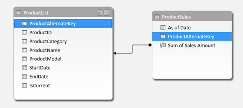
By loading the ProductSales.xlsx table, we now arrive at the following dimensional schema:

image

generated SCD Type 1 dimensional schema

With the following result:

image


GROWTH STAGE #2:  MOVING TO RELATIONAL SOURCES

Once the model is proven popular and useful to the business,  the BI team may decide to take the ETL prototype query and standardize it in a SQL view:

CREATE VIEW [dbo].[v_ProductList] AS
SELECT       
        ProductList.*,
        ProductSales.[Product Name],
        ProductSales.[Product Model]
FROM           
        ProductList LEFT OUTER JOIN
        ProductSales ON ProductList.[Product ID] = ProductSales.[Product ID]
WHERE       
    ProductSales.[As of Date] =
    (
        SELECT MAX(ProductSales.[As of Date])
            FROM ProductSales
    )
GO

Notice the pattern used would be very similar to the one used to create a valid dimension (lookup). In the model, we can now change the connection to point to this view and get rid of the Excel source dependency. To do this, we must change the connection used to populate the tables from a file source to a SQL Server source.

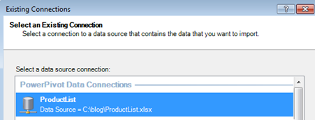
Go to ‘Existing Connections’j, select ProductList.

image

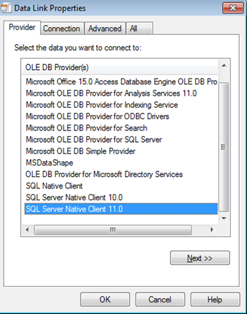
By clicking ‘Edit’, it is now possible to change the connection type by clicking ‘Build’.  When the ‘Data Link Properties’ window opens, change the provider to ‘SQL Server Native Client 11.0’.

image

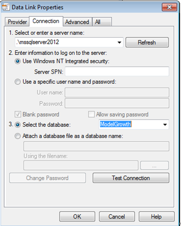
At this point, you can connect to the SQL Server source and specify the database that contains the extracted datasets.

image

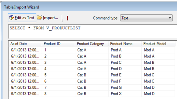
Once the connection is mapped back to SQL Server, we must change the query definition that makes up the ProductList. This can be done in using the ‘Table Properties’ option of the model.

image

Given the maturity of the implementation, it may be advantageous to upgrade the PowerPivot model to BISM Tabular, while also developing more sophisticated ETL.


GROWTH STAGE #3:  ENABLING HISTORICAL TRACKING

The business may decide it would be beneficial to enable historical attribute tracking to create more sophisticated reporting.   At this point, we can use a variation of the query we have discussed in order to initialize a target data warehouse dimension “DimProduct”.

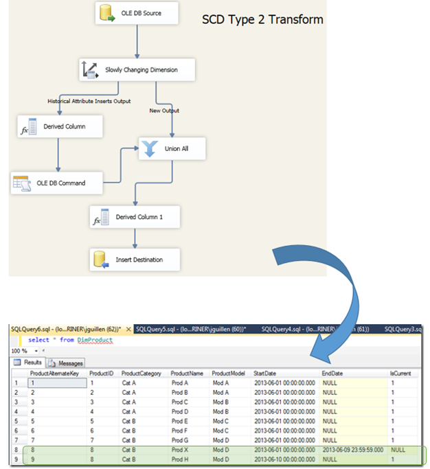
SQL Server Integration Services could now fulfill that exact requirement, but producing the more complex transformations to record attribute changes over time. 
 

image

Once the SCD Type 2 transform has been defined, it is important to re-map the Tabular model to use surrogate instead of natural keys as part of the relationship.  This can be simply done in the PowerPivot or Tabular model design interface:

image

generated SCD Type 2 dimensional schema

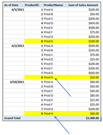
The result is a model that grew from simple file sources to a more sophisticated environment leveraging appropriate data transformations.

image

The process described is not a theoretical one but is based on real scenarios I have seen evolving without much effort, as each step fuels the project further. In my opinion, this makes up for great “BI”, as nurturing model growth allows us to stay relevant by developing close to the business, and in turn ensures accuracy and strong sponsorship on the projects implemented.

PivotStream and Mariner join forces to deliver PowerPivot solutions

I am excited to share the news that PivotStream, the world’s leading provider of hosted PowerPivot solutions, and Mariner, the company I work for in which I help device PowerPivot solutions and practices, have entered into a partnership agreement to provide services that leverage our complementary skills and expertise.
image

It is my hope this partnership will speed up the propagation of the the PowerPivot story as we help organizations take advantage of the strength behind business-driven data discoveries. Our goal is to help Excel analysts generate critical business impact in decision making, despite tightly I.T. controlled regulations on data production and consumption.
I am looking forward to help take our clients to the next level of business agility !!! 🙂

Configuring “drill to details” behavior in PowerPivot: Part 1

It has been said there is no way to change the default drill through behavior in PowerPivot.  However, if we look closely we discover that we can actually exercise a bit more flexibility than normally assumed when using this feature.

The first thing to understand is that drill through retrieves data from whichever table the measure has been assigned to.

This is an interesting feature – yet, not very intuitive –:  as it is possible to assign a DAX measure to any table in the model (even disconnected ones) without affecting the output of the measure at all, one can allocate measures to tables specifically designed for drill through.

Lets look at an example using Adventure Works.

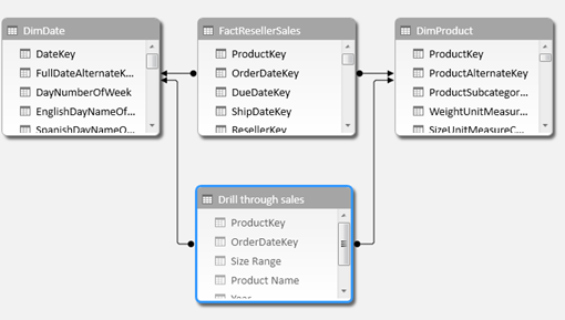
image

[Sum of SalesAmount] is an implicit measure.  As such, it was allocated to the table with numeric values (FactResellerSales). Notice this table is on the many-side of the context propagation.  When executing a drill through, we get an ‘exploded’ view of that table showing raw data:

image

Also notice that many technical columns are retrieved, which may not provide any value to the analyst (ResellerKey, for example) .  Instead, lets create a custom table to support a more customized drill through view, with only the columns we are interested in.  I will use the Table Import Wizard instead of writing straight SQL, as I believe this is something analysts will be able to configure on their own without the need to code:

image

By specifying the use of ‘Group and Aggregate’, we will get a list of the distinct product and order date keys in our fact table. As we might not interested in the original granularity as we are simply supporting a drill through action in order to show what dimension members make up a specific sales amount, a list of product and date members is sufficient in this case.

image

We can source the desired columns from the lookup tables by using RELATED. Or, to save memory space or for model usability, you may decide not to bring those columns on the visible lookup tables and only retrieved them from the source to populate the custom drill through table.

All columns should be hidden (do not hide the table, only the columns.  Hiding the table will hide the measure we will assign to it which is not what we want).

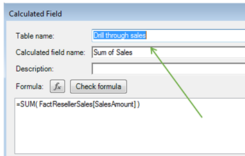
An explicit DAX measure is created at this point:

[Sum of Sales]:=SUM( FactResellerSales[SalesAmount] )

and assigned to the ‘drill through sales’ table:

image

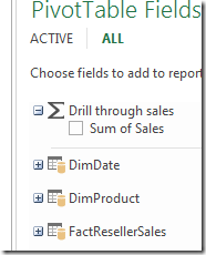
As only the measure is visible on this table, the pivot table field list will not show the regular table icon but one indicating the summation sign:

image

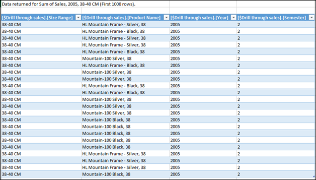
When clicking on the cell we clicked before, this time we get a more ‘customized’ drill through:

image
Note the keys connecting to the related tables are hidden, they are never retrieved on the drill through view.  This is good, as they are technical and not needed for analysis.

The order of the columns depends on the order in which you added the RELATED columns on your custom drill through table.  Simply moving the column to another position won’t change it on the drill through view.  To change order, it is necessary to re-create the order you wish to see.

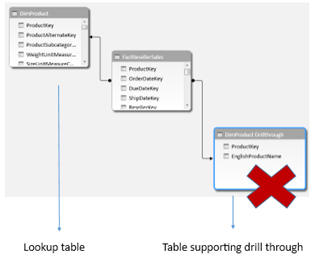
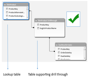
In order to custom drill through views to work, the default context propagation (from the one-side to the many-side) must be respected. As such, if you want to provide a small drill through experience from the visible lookup table you should snowflake the model instead of connecting both tables (visible lookup and custom drill through) to the fact table separately:

image      image

Note: in Excel 2013, there appears to be no way to change the default behavior of 1000 rows retrieved (this was not the case in Excel 2010).

Developing child-aware KPIs in PowerPivot and BISM Tabular

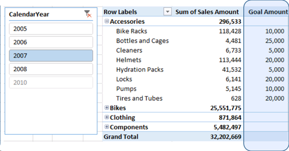
Sometimes you want to see if a parent level has violated a target value based on a comparison at the child level.  For example, you want to browse a dashboard showing Product Categories and visually indicate which of those categories had Product Subcategories that violated a designated sales quota.  Note that the quota is not assigned at the Product Category level, but the Subcategory level instead .

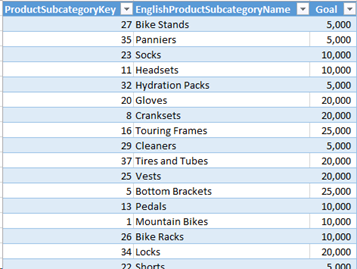
So we first must be sure to create a DAX expression that will decisively compute at the child level desired.  In the example above, the target quotas would look like:

image

I am only showing a few of them but I hope the point is clear (also, for simplicity, I have not defined goal amounts per year, which is certainly doable).

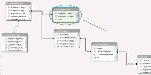
For any given subcategory, we have a determinate ‘goal’ or target sales quota.  As this table is now just a lookup in the model, we can connect it to the dimension with appropriate granularity (DimProductSubcategory)

image 

The expression needed to see what we are comparing against at the Subcategory level is:

Goal:=If (
  ISFILTERED ( DimProductSubcategory[EnglishProductSubcategoryName] ),
  If (
    Sum ( FactResellerSales[SalesAmount] ),
    Sum ( SubcategoryTargetAmount[Goal] )
  )
)

The output of which is:

image

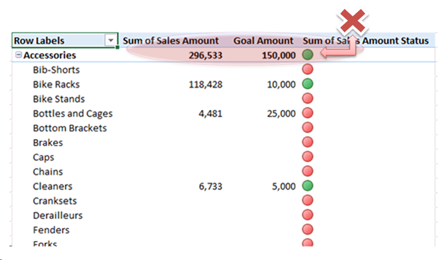
At this point we could think about using built-in KPI capabilities.  In this scenario, however, this would not be helpful as KPIs, by default, compute at the level of granularity displayed and they also include subcategories even if the is no sales or goal data for them:

image 

In the screenshot above, I removed the ISFILTERED condition of the Goal Amount DAX expression so it will show a value at the parent Category level. Notice that the status is green as the comparison – at that level – is favorable.  This is *not* what we want:  instead, it should be flagged as RED when any child level violated the goal amount (which is the case of the Accessories category shown). 

In addition to that, and as mentioned before, note that the KPI is computed for all subcategories, whether they have sales and goals amount or not: again, not ideal.

Instead, we will be creating our own custom KPI.  As such, there is a need to compute the ‘status’ value on our own  through a DAX expression:

KPI:=If (
  ISFILTERED ( DimProductCategory[EnglishProductCategoryName] ),
  SumX (
    Values ( DimProductSubcategory[EnglishProductSubcategoryName] ),
    If (
      [Sum of Sales Amount],
      If ( [Sum of Sales Amount] < [Sum of Goal Amount], – 1, 0 )
    )
  )
)

The expression always computes at the Subcategory level (even at the Category level).  It then rolls-up the amount of children that violated the goal (each of those will be assigned a value of –1).

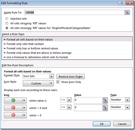
When consuming the model through a pivot table, we can then use conditional formatting to mimic a regular KPI:

image

Notice that the rule is applied, not to a cell range, but to a measure (KPI).  Also, the value assignment per icon may look a bit strange as it is designed to work with three value bands whereas here we only have two (negative or zero). 

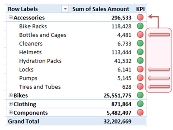
The final output properly display parent level alerts based on children level violations:

image

Its interesting to point out that event though there is 4 children that complied to the KPI rule and other 4 that did not, the parent level category does not “net out” the result.  This is an important distinction and the reason why the DAX expression uses 0 for positive values instead of 1.

Grouping by an Aggregation in DAX

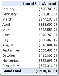
Business users really like the option of comparing category members against the average for all. Let’s review how to accomplish this in DAX.

image

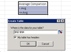
Suppose you what to find out which months had an above average sales performance on the data above (tables come from AdventureWorksDW).  We must first create a new table in the model, to hold the categories we want. In PowerPivot, these values can imported as a linked table:

image 

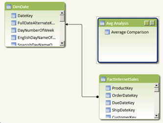
The resulting model is the following:

image

As sales data is per day, but we want to find out the monthly average, we must use an expression that computes this aggregate at the correct level of granularity:

image

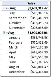
With this, we can now use a measure leveraging a conditional DAX statement to categorize the monthly output as needed:

image

Notice here we also compute at the monthly grain by use of the SUMX function iterating over the list of unique month names. This is important in order to allow for proper aggregation at the subtotal level.

image

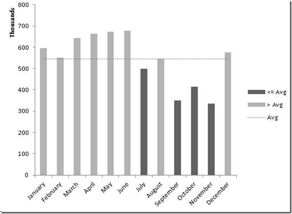
The data model allows now to create an interesting visualization, using color as an indicator, to emphasize those months that are below average (to graph the dotted line, I added one more value to the linked table to allow for display of the computed average value itself):

image

Grouping on Quartiles

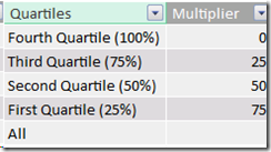
Another interesting example of is grouping data by quartiles.  In order to do this, I modified Colin Banfield’s quartile DAX expression to dynamically compute based on the “utility” linked table which has no relationships with other tables in the data model, and contains the needed multipliers to compute at each percentile value.

image

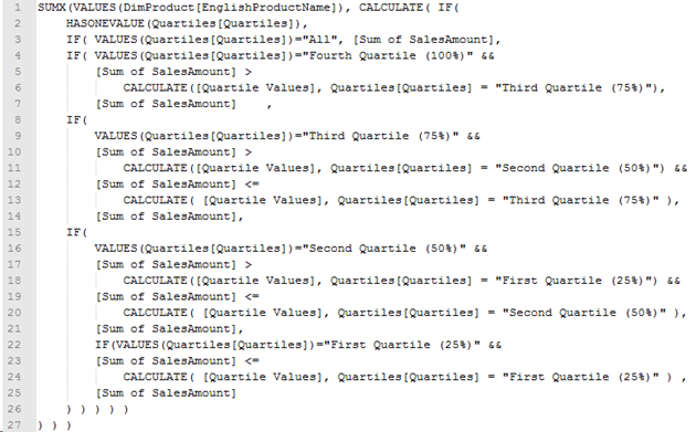
A final expression allocates the sales amount to the appropriate quartile column, and ensure the computations happens at the product level:

image

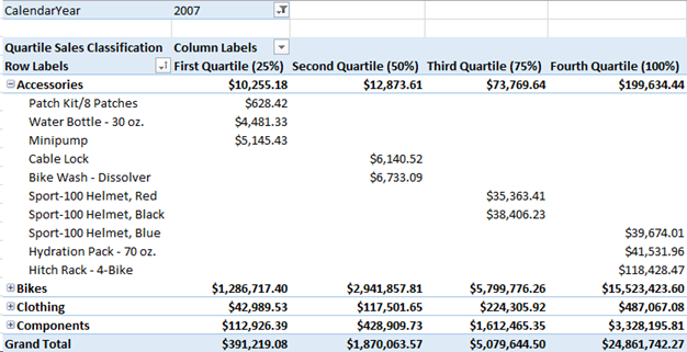
Here is the result:

image

Notice that subtotals are computed on quartiles appropriate for the current category in the filter context.  Same applies to the grand total.

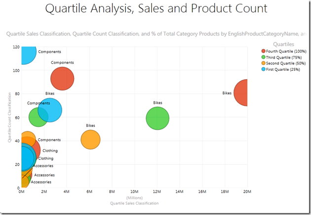
In Power View, I cross referenced the sales amount (on X axis) with two additional, quartile based metrics: count of sold products per category (Y axis) and % sold products over all available category products (bubble size). 

You can see that the “Component” product category had lots of sold products (out the entire category) on any given quartile, however “Bikes” had more products with sales on the 4th quartile than it did on the second or third, and overall was the most profitable category.

image

Leveraging DAX query tables for staging Data Transformations

When designing a data warehousing solution, it is typical to allocate certain data transformations to the ETL layer, particularly those that would be easier or more efficient to do outside of the cube.  At the same time – prior to Excel 2013 release – developing multi-step data transformations in a Data Model was, whenever possible, a factor that increased the complexity (and lowered maintainability) of DAX formulas.

Interestingly though, using DAX query tables – a feature Kasper de Jonge blogged about some time ago here – we now have the ability to generate materialized intermediate tables that can be consumed back into the Data Model, allowing us to generate a process that includes not only a semantic layer but a degree of automated data transformations.

So, as an example, here is what we are going to do:

image

To be clear, the output of the transform (the intermediate or *staging* table) also lives in the Data Model.  Nevertheless, those of you familiar with the data warehousing process will notice a similarity to a typical integration process. Also note that I used linked tables here for simplicity, but other sources are possible as well.

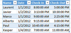
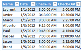
The goal is to take the table below (‘Check-Ins’) and generate a report that breaks down total full hours versus partial hours worked on a daily basis.

image 

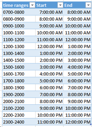
As you notice, data is not currently in a way in which is easy to count how many full or partial work hours where recorded.  It would be easier to un-pivot this data, and cross join it with a reference table to break it down by hours. As such, the following generic and re-usable lookup table (‘Time Ranges’) should be added to the Data Model:

image

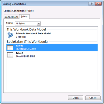
After importing them as linked tables, we then generate a place-holder table from any of the tables in the model.  This can be done, from Excel, under Data –> Existing Connections – > Tables Tab:

image

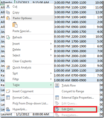
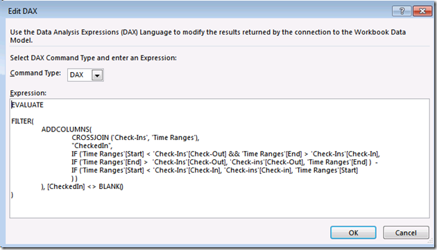
At this point, a DAX transformation query can be used to generate a new output.  Right clicking on the table generated gives us the option to edit the DAX query used to generate the intermediate (or staging) table. We are interested in seeing, for each person in the source table, the break down of full and partial hours.  Here is the query (thanks to Laurent C for the ideas on this particular data transformation):

image

                                image

image 

                                                                                   image

image

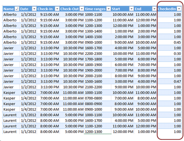
This table breaks down the full and partial hours worked per person.  It can now be re-imported into the Data Model, and enhanced with additional calculated columns:

CalculatedColumn1 ( FullHours)

=IF([CheckedIn] = "12/30/1899 1:00:00 AM",1)

CalculatedColumn2 (PartialHours)

=IF([CheckedIn] <> "12/30/1899 1:00:00 AM",1)

Out of which two fully additive measures can then be generated:

image 

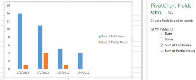
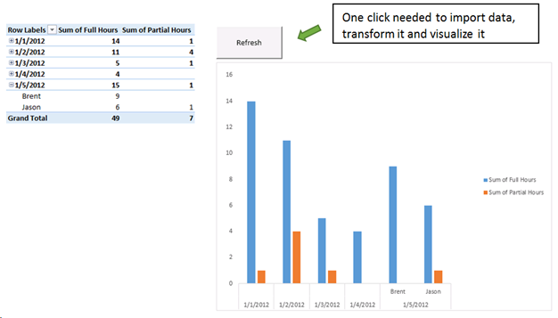
With data from this intermediate table, the final report is now easy to create:

image

DAX query tables are great but they don’t – by themselves – offer a way to solve an important question:  The sequencing needed to compute the output.  In addition to that, we have the issue of the amount of data refreshes needed:

image

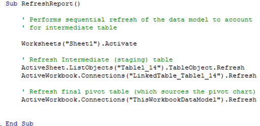
Coding against the sheet object model, however, we can consolidate the refreshes into one while controlling the order of execution required by the calculation.  This is what makes the solutions so similar to an ETL process. We get one button control that can:

1) import all changes from the linked table sources

2) refresh the intermediate DAX table query and

3) reflect the changes on the report, in one pass while controlling the other of execution.  Here is the code:

image

New data can be added to the linked table source, and by clicking on a button (with the VBA RefreshReport macro assigned to it), one can perform the sequential refresh needed for the Data Model to consumes itself in the staging table.

With the particular scenario used here, the whole computation could have been done in a single DAX expression, however, this approach would prevent reusability of the staging table, having to recomputed it again for each measure as it is not materialized.

[Notice Jason and Brent have been added to the source linked table]

image

                                image 

image

An outstanding question remains on how to move these ‘Personal BI’ initiatives into a wider Enterprise model.  It is still necessary to consider BISM Tabular models strip out the Excel dependency of imported PowerPivot models, yet this technique requires that exact dependency to be present.

This article is a companion to Jason Thomas’ most recent blog entry, which uses this technique to generate a data model that allows for cross-dimension filtering.