SCOPING at different granularities in DAX (Part III)

In the last two blog entries on this topic (available here and here), we got a bit closer to reproducing – in DAX – the same output one would normally achieve with the MDX scope statement.

In this new entry, we perfect the formula a bit more by ensuring filter context propagates to the higher levels of granularity we are affecting.  Thanks to Gerhard Brueckl ( blog ) and Jason Thomas ( twitter | blog ), who contributed greatly to this blog entry and helped point out areas of improvement.

With the last formula we used, we are able to retain the Fiscal Quarter context (and split its value evenly among the months that belong to it), even if fiscal quarter is not part of the query context.

There is one issue with the formula, though:  if a user modifies the query context to include only two months for example, each belonging to a different quarter, the total for the year would be incorrect.  Let’s take a look:

If we manually add the quarter totals we can see the fiscal year value is off.   What is happening here?  We must realize that we are ‘scoping’ at the month level: through the use of

SUMX ( VALUES ( <month> ), <expression invoking fiscal quarter> )

we are:

1. iterating over a list of monthly values and
2. making a reference to the quarter(s) at the current filter context

With this understanding we can now see how at the Fiscal Year level the context will contain two quarters.  As such, each iterated month will be accounted twice.   The solution is a VERY simple one, yet not immediately intuitive:   We must wrap our CALCULATE expression with another CALCULATE.  In this way, the ‘current month’ in context will only refer to the actual fiscal quarter that contains it – avoiding ‘double counting’ of data.

Here is the final expression:

Scoping v3 (SUMX):=SUMX(
    VALUES( DimTime[EnglishMonthName] ),
    CALCULATE( CALCULATE( SUM( FactSalesQuota[SalesAmountQuota] ) ,
            ALL(DimTime[EnglishMonthName]),
            SUMMARIZE(DimTime, DimTime[FQ] )
        )
    /
            CALCULATE( DISTINCTCOUNT( DimTime[EnglishMonthName] )  ,
                ALL(DimTime[EnglishMonthName]),
                SUMMARIZE(DimTime, DimTime[FQ] )
            )
) )

Notice the double CALCULATE on the third line.  We are:

1) computing an expression based on modified filters (the first CALCULATE) and then…

2)  converting row context into filter context so each Month gets assigned the appropriate value (the second CALCULATE).

Whenever you are “scoping” at a specific level in DAX, you must use a double CALCULATE pattern in order to propagate context appropriately at levels higher than the one you are currently affecting.

With this change, context now gets properly established at the year and grand total levels:

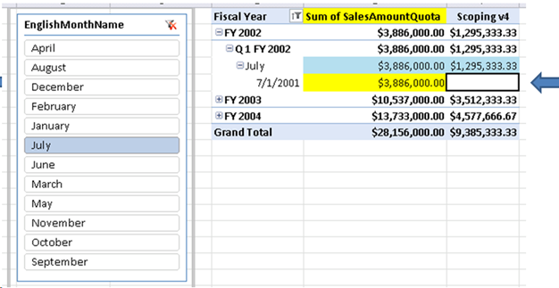
Finally we must consider not only the levels above month (quarter, year), but also the levels below (day).   As shown in the first part of this blog series, the SSAS cube dimension usage is assigned, in Adventure Works’ Sales Targets measure group, at the quarter level of granularity.  This in effect leaves date level members with no sales target values (even though the actual relationship happens at the daily grain in the DSV):

We can modify the DAX calculation to mimic the same behavior.  Instead of modifying the Tabular model itself, we can simply add a condition to our calculation so it will only execute at monthly levels and above, but never at the daily level:

Scoping v4:=SUMX(

    VALUES( DimTime[EnglishMonthName] ),

    CALCULATE(IF(NOT(HASONEVALUE(DimTime[FullDateAlternateKey])) ,

            CALCULATE(

                SUM( FactSalesQuota[SalesAmountQuota]) ,

                SUMMARIZE(DimTime, DimTime[FQ] ) ,

                ALL(DimTime ) /

            CALCULATE( DISTINCTCOUNT( DimTime[EnglishMonthName] )  ,                

                SUMMARIZE(DimTime, DimTime[FQ] ),

                ALL(DimTime)

                )            

            ) ) )

 

Notice the only change in the calculation is the IF statement on the third line.  With it, we now are able to fully match MDX behavior at any level of a Calendar hierarchy.  If you are in need to compute a DAX expression at a specific level of granularity on your Tabular model, consider using a similar pattern as the one exposed above.

Finally, if we want to simplify this pattern we can replace the outer CALCULATE with SUMMARIZE.   As both of them have the ability to turn row context into filter context – which is needed to accurately compute at all levels – we can use it to generate a more readable version of the calculation – Thanks Gerhard for the suggestion!

SUMX(

SUMMARIZE(DimTime, DimTime[EnglishMonthName], "CalculatedMonthValue",

IF(    NOT(HASONEVALUE(DimTime[FullDateAlternateKey] ) ),

CALCULATE(

        SUM(FactSalesQuota[SalesAmountQuota])/DISTINCTCOUNT(DimTime[EnglishMonthName]),

        VALUES(DimTime[FQ]),

        ALL(DimTime))) ),

[CalculatedMonthValue]
)

SCOPING at different granularities in DAX (Part II)

As mentioned on the prior post on the topic (available here), the DAX calculation that mimics MDX scope behavior requires a certain ‘filter arrangement’ to work properly.  In other words, it actually expects a display hierarchy -  otherwise it will not yield the correct results. Can we overcome this to more closely resemble MDX behavior? Interestingly, yes – is it possible, using a variation of the formula exposed on the prior entry.

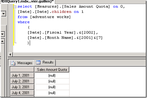
Let’s examine this issue a bit closer:  Continuing with the MDX scope Adventure Works example which was used in the last blog entry, I am able to query the month directly and still get the assigned cell values even if the quarter is not part of the query expression:

With the DAX solution we used, however, we are unable to get the same results as we expect to Fiscal Quarter to be part of the current query context. Lets first remember the correct output.  Notice we are using a fiscal hierarchy of year, quarter and month:

As you may recall, the calculation limits itself to clearing the filter context on month (highlighted below), which forces the engine to use the next display hierarchy level available to allocate the calculation context. This happens to be quarter in our example. Once we grab that value, we split it by the number of months belonging to that quarter:

SUMX(
    VALUES(DimTime[EnglishMonthName]),
    CALCULATE(
        SUM( FactSalesQuota[SalesAmountQuota]  ) / CALCULATE( COUNTROWS( VALUES( DimTime[EnglishMonthName] ) ), ALL( DimTime[EnglishMonthName] ) ), 
       ALL( DimTime[EnglishMonthName] )
    )
)

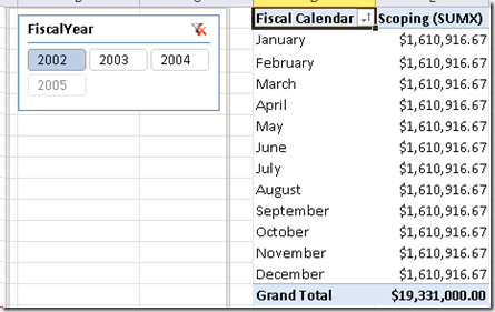
If we remove the quarter from the query context, we get:

Clearly not matching MDX results. So how can we truly assign a value derived from a quarter level assignment to the monthly level, regardless if quarter is in the resultset or not? One way of doing this is by leveraging the SUMMARIZE function.  With it, we can build a table on-the-fly at the appropriate level required and use it as a ‘set filter’ parameter to the CALCULATE function:

Scoping v2(SUMX):=SUMX(

    VALUES( DimTime[EnglishMonthName] ),

        CALCULATE( SUM( FactSalesQuota[SalesAmountQuota] ) ,

            ALL(DimTime),

            SUMMARIZE(DimTime, DimTime[FQ] )

        )

    /

        CALCULATE( DISTINCTCOUNT( DimTime[EnglishMonthName] )  ,

            ALL(DimTime),

            SUMMARIZE(DimTime, DimTime[FQ] )

        )

)

Notice that Fiscal Quarter ([FQ]) is called within the SUMMARIZE function.  As such, the calculation will always use fiscal quarter values, regardless if fiscal quarter is used or not in the query context. This is not too different from the MDX Scope definition used in Adventure Works:  on it, a reference to the Parent level of the CurrentMember is used, and as the Scope is defined for the Month level, the resulting output always takes the Quarter into consideration.

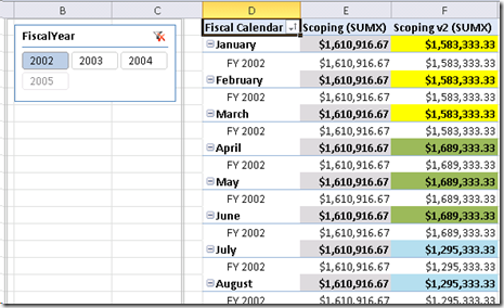
The resulting DAX output matches MDX Scope:

The pattern of - 

^{AggregateX( <granularity at which the expression executes>, <expression>)}

is still being used here.  So for each cell output displayed, the calculation always executes at the monthly level of granularity even if what I am showing is quarterly or yearly data.

In order to ensure the pattern works, lets test a few more things.   First, lets add the Fiscal Year below the month:

We see that the new calculation (Scoping v2), is able to keep its context appropriately even in this scenario.

As a second test, lets place the Calendar Year and Calendar Quarter in the row labels instead of the Fiscal Year and Fiscal Quarter.   With the initial calculation, the current query context will dictate what will be used to compute the monthly values.  However, as the new calculation explicitly calls the Fiscal Quarter as part of the expression, the values will still be correct even in this case.  In order to make the solution easier to understand, I added an extra measures called ‘Current Fiscal Quarter’ to the model with the following definition:

Current Fiscal Quarter:=IF(HASONEVALUE(DimTime[FQ]),

                                                   VALUES(DimTime[FQ]) )

Now, if we place the Calendar Year and Quarters in the row labels, we get:

As you can see, monthly values are still evenly assigned from the Fiscal Quarter, even though the fiscal quarter is not part of the slicing hierarchy at all.

As mentioned on the prior post,  Jason and I will be using a similar pattern to tackle some interesting Last Non Empty Scenarios.  That, however, will be the subject of a future post

SCOPING at different granularities in DAX (Part I)

One of the most powerful MDX functions is SCOPE.  With it, one can override cell values at any level of granularity in an SSAS cube and their new custom values will now be considered when returning aggregate results.

It is generally understood you can’t use SCOPE-type functionality in an SSAS Tabular model.  But if we examine the topic a bit closer, we realize that a lot of what is possible with SCOPE statements can also be replicated with DAX expressions.

One of these examples is the ability to manipulate the granularity at which a computation executes.   My colleague Jason Thomas ( blog | twitter ) recently posted a blog entry of a technique in which the expression scope is changed in order to iteratively prototype the correct granularity needed for a business calculation (See his blog entry here). This is the same technique can also be used to solve advanced Last Non Empty scenarios, something we will blog about soon.

Lets look at another example.  In the Adventure Works cube, there is a SCOPE statement in the MDX cube script in which months are evenly assigned the sales amount quota of their parent quarter on the fiscal year 2002:

In the cube designer we see that this is necessary in order to have monthly values, as the dimension usage has been defined by tying the ‘Sales Targets’ measure group with the Date dimension at the Year/Quarter level of granularity:

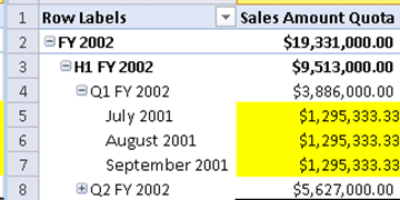
When browsing in Excel, we see the output of the behavior as:

We can achieve the same behavior on a tabular model by iterating through the distinct list of months in the lookup (dimension) table. To begin with, we load the appropriate tables in the tabular model:

Note that I created a hierarchy with custom fiscal year (FY) and fiscal quarter (FQ) calculated columns, in order to match the dimension member caption in the Adventure Works cube. When pivoting the data, without any DAX expressions defined, we get:

Notice the sales amount quota is tied to only one month.  This is because DimTime is at the daily level or granularity;  when Fact Sales Quota relates to DimTime, it assigns values on a specific date – however, as these quota values have been defined by the business at the quarter level, the regular sum aggregation at the monthly level does not make much sense.

SCOPE, in the MDX cube script, deals with it by getting the quarter value and dividing it in three, and assigning this new value to each of the months belonging to that quarter. To match the output of MDX SCOPE in a Tabular model, we use the following DAX expression:

Scoping (SUMX):=SUMX(

    VALUES(DimTime[EnglishMonthName]),

    CALCULATE( SUM( FactSalesQuota[SalesAmountQuota]  ) /

            CALCULATE(

                COUNTROWS( VALUES( DimTime[EnglishMonthName] ) ),

                ALL( DimTime[EnglishMonthName] ) ),

        ALL( DimTime[EnglishMonthName] ) )

)

Which yields the following output:

This DAX pattern involves using a row-by-row execution using SUMX over a table of distinct values at the desired level of granularity:

AggregateX ( <granularity level>, <expression> )

As you see, the pattern is just using the signature of any of the AggregateX functions.  The only difference is one of perspective:  in our case, we are explicitly leveraging the first argument to change the granularity at which the expression evaluates.  The granularity level is specified by generating a table at the appropriate level desired, whether you use VALUES, SUMMARIZE or even CALCULATETABLE.

This same technique is something Jason and I have explored when tackling interesting analytical scenarios, like the calculation of Last Ever Non Empty, which also uses the same pattern.

Clearly, the same result can be achieved by using other methods in this case.  One of those is by detecting level, as explained in more detail on prior blog entry.  If we apply that technique here, we get:

Scoping (ISFITLERED):=IF(

    ISFILTERED(DimTime[EnglishMonthName]),

        CALCULATE(

            SUM( FactSalesQuota[SalesAmountQuota] ) / 3,

            ALL(DimTime[EnglishMonthName] )

        ) ,

    IF(

        ISFILTERED(DimTime[FQ]),

            SUM( FactSalesQuota[SalesAmountQuota] ) ,

    IF(

        ISFILTERED(DimTime[FY]),

            SUM( FactSalesQuota[SalesAmountQuota] )

        )

    )

)

Notice how the total level is not showing a value, as I didn’t account for that level in my conditional IF statements. This is not ideal as in many scenarios you need the ability to compute on a level that is not displayed on the pivot table or report.

For example, if we wanted to slice this measure by  the Sales Territory Group dimension, we would get:

As you can see, when an unexpected context has been introduced, the technique using SUMX is still able to compute at other levels whereas using ISFILTERED can’t due to the unexpected filter which is not accounted for. Clearly, using ISFILTERED in this case would diminish the usability of the model.

ANATOMY OF THE CALCULATION

As we are computing rows for each member at a specific level or granularity, it is necessary to iterate through this members. The SUMX function allows us to do just that.

It is known that iterative functions like this do not perform as well as other calculations that compute on ‘bulk’ mode (like SUM).  However, SUM can only take a column for parameter, whereas with SUMX we can specify a table on which the expression will be computed on a row-by-row basis. An we need this table parameter precisely because it is the one that allows us to define the grain at which we the evaluation to be evaluated.

The calculation takes the list of distinct months and, through row context, grabs the quarter value and divides it by the count of months belonging to that quarter.  This is possible due to the fact that the context at the month level has been cleared out, and hence the values always belong to  the next level for which there is context (quarter in this case):

Notice also that the distinct list of months must be generated off the appropriate side of the one-to-many relationship:  if we had a column for month on the fact table and used that we would have gotten the following, obviously incorrect results:

Scoping (Incorrect Grain):=SUMX(

   VALUES(FactSalesQuota[FactMonth]),

    CALCULATE(

        SUM( FactSalesQuota[SalesAmountQuota]  ) / CALCULATE( COUNTROWS( VALUES( DimTime[EnglishMonthName] ) ), ALL( DimTime[EnglishMonthName] ) ),

        ALL( DimTime[EnglishMonthName] )

    )

)

Clearly, values not assigned on all qualifying months – only the ones active based on query context. As I have described on a prior blog post, DAX context does not automatically propagate from the base table to the lookup table.

We can take advantage of this by generating the distinct list of months based on the lookup table: doing so guarantees we will get a list of all months, regardless of the current filters in action on the fact (base) table.

IS THIS A REAL ASSIGNMENT OF VALUES?

It is not. In DAX, we are not really assigning or overriding values as we would with an MDX scope statement.  However, in Tabular, we have the ability to generate a new calculation that computes at a certain level of grain; this allows us to mimic the same behavior as that achieved through MDX.

The experienced MDX or DAX user may have noticed that our defined calculation expects a hierarchy in order to show the assigned values: we do this as we are clearing some filters but expecting others to be kept. When looking at the results at one level of grain only (monthly), this will lead to different results to those we get by use of the MDX SCOPE function. However, using DAX we are able to overcome this: see how on the second blog entry on this topic available here: https://javierguillen.wordpress.com/2012/05/04/scoping-at-different-granularities-part-ii/