Creating a custom unknown member in BISM Tabular

One nice feature that UDM / Multidimensional SSAS cubes have is that of being able to specify a custom name for the ‘unknown’ member – that is, the member automatically generated by the presence of foreign keys in a fact table that refer to members not present in the dimension table.

In Tabular, the default behavior is to assign a blank member. We can easily see this with an example:

DimProduct:

FactResellerSales:

Notice there is a ProductKey that is present in the fact table, yet missing in the dimension (ProductKey 216). This could be the case due to late arriving dimensions.  In any case, when pivoting this data, the default behavior is the following:

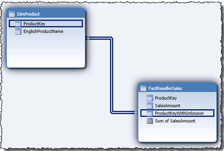
In order to assign a custom name to the unknown blank member, we must first assign a new unknown member to the dimension table and then generate a new calculated column in the fact table that will be used to establish the relationship.

For relational data sources, select the dimension table and then click on ‘Source Data’ on the properties window.  Be sure the drop down on the top right says ‘Query Editor’.  If not, switch from ‘Table Preview’ to ‘Query Editor’ in order to manipulate the query.  Then UNION the query with a row with ‘unknown’ values, for example:

We must delete the existing relationship as we won’t be using the same column to recreate the relationship with the custom unknown member.  Then, add a calculated column on the fact table that generates a lookup on the dimension and when unable to find a value, output a  “-1”: As the relationship won’t be there, we cannot leverage the RELATED function anymore, it must be done via a CALCULATE statement:

FactResellerSales[ProductKeyWithUnknown]

=IF( CALCULATE(
        COUNTROWS(DimProduct) ,
        FILTER(DimProduct,
        DimProduct[ProductKey] = FactResellerSales[ProductKey]) ) = 0,
    -1,
      CALCULATE(
        MAX(DimProduct[ProductKey]) ,
        FILTER(DimProduct,
        DimProduct[ProductKey] = FactResellerSales[ProductKey]) )
    )

Note that using MAX(DimProduct[ProductKey]) instead of VALUES(DimProduct[ProductKey]) as part of the calculation is necessary to avoid circular dependency errors when establishing the relationship. Having said that, we can go ahead and create this relationship between this new calculated column and the dimension key column.

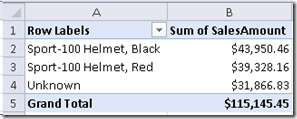
That’s all.   Pivoting the data, should now look like this:

Though the approach may avoid the need for ETL in this kind of operation, a downside is that the Product Key is being stored twice.  For really big tables, it may be worth exploring the ETL option in order to keep memory as tight as possible and avoid the need to duplicate columns.

Speaking for PASS Business Intelligence Virtual Chapter

On March 27, I will be speaking for the PASS BI VC on “Transitioning from Self-Service BI to Corporate BI:  PowerPivot & the BISM Tabular model“.

If you are interested in learning more about how to increase the reach and accuracy of Corporate Business Intelligence initiatives by leveraging the data discoveries achieved through self-service analytics then I think you will be enjoy attending my presentation.

To learn more about it, visit the Virtual Chapter website @ http://bi.sqlpass.org/

OFFSET double lookup in PowerPivot

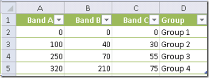
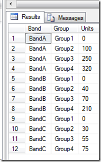
One of those really great functions in the native Excel environment is OFFSET.  In combination with other functions like MATCH, it can generate a type of ‘double lookup’ that can be really helpful when creating dynamic reports.  For example, the table below describes a matrix defining a coordinate of units for each combination of ‘Band’ and ‘Group’.

We want to use this table as a lookup reference when generating matches for the following values:

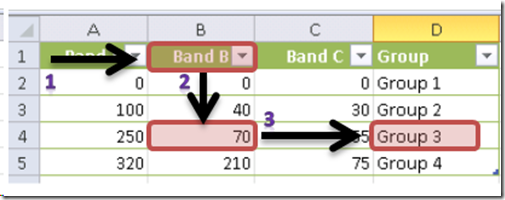
Take for example, the first row.   We first look at the ‘Band’ value which is B in this case and find it in our lookup table.  Then we go down the rows and, using an approximate match logic, find the group for which the value of 120 belongs to.   That would be Group 3 (which has unit values going from 70 to 129).

In Excel, we can use a formula like the one below to generate this ‘double lookup’ calculation:

VLOOKUP(A11,

OFFSET($A$1,1,MATCH(B11,$A$1:$D$1)-1,4, 4),(4 – MATCH(B11,$A$1:$C$1)) + 1,TRUE)

This formula finds the appropriate columns first (column B) and then uses an approximate match VLOOKUP to find the row (#4) and column ( D ) to retrieve the right group.  The final result is:

Pretty powerful.

If we are analyzing data with PowerPivot, we want to be able to generate the same effect within the PowerPivot itself without having to drop all data into Excel and do the OFFSET lookup there. This could be because we are scanning millions of rows or simply because we want to keep all calculations in the same place (the PowerPivot database)

In order to do this we need to first understand one thing: we must unpivot the lookup table so we can successfully generate the lookup in DAX.   Unlike what you can do with the OFFSET function – in which you can specify a column / row coordinate dynamically – in DAX we will be only filtering rows.

If our data is in a database like SQL Server, we can do this by executing the following T-SQL expression:

SELECT Band, [Group], Units FROM

    (SELECT BandA, BandB, BandC, [Group] FROM Table1) t

UNPIVOT

    (Units FOR Band IN (BandA, BandB, BandC)) as unpvt

ORDER BY Band, [Group], Units

The result will be the following:

In the case you are relying on data which resides only on your spreadsheet, you can use the ‘Multiple Consolidation Ranges’ wizard to generate the same effect.  This wizard is found by going to File –> Options –> Customize Ribbon.  On the ‘Choose Commands From’ dropdown, select ‘All Commands’ and then find and add to your ribbon the ‘Pivot Table and Pivot Chart Wizard’.  Finally, click on the wizard button we just added to the ribbon.  You should see the following window:

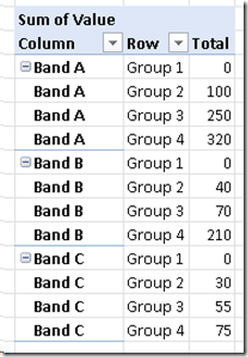
Notice that I moved the ‘Group’ column to the left. This is because the wizard expects the categories on the first column. Select ‘Multiple consolidation ranges’ and follow the instructions.  Once complete, you will get a pivot table using the data from our lookup table. Move the ‘Row’ and ‘Column’ fields to the row labels.  Finally, flatten the table out (using the PivotTable Options context menu) and you will end up with the following result:

Now you are ready to import the unpivoted lookup data into the PowerPivot window.  Be sure to change the column names to something more meaningful than ‘Column’, ‘Row’ and ‘Total’.  In my case, I have called them ‘Band’, Group’ and ‘Units’.

Finally, import the items that we are going to be using against the lookup (2nd screenshot on this blog entry) – I called it ‘Data’. Notice that this is yet another scenario in which there is no actual relationships between the tables in the data model. All the work will be done using a DAX expression:

DoubleLookup:=IF ( HASONEVALUE( Data[Band] )  ,

CALCULATE(

        LASTNONBLANK( Lookup[Group], 1) ,                   

                       FILTER( Lookup,

                        Lookup[Band] = VALUES(Data[Band] ) &&                     

                        Lookup[Units] <  VALUES( Data[Units] )

                    ) 

            )

)

Notice the expression is very readable and shows how a fairly simple DAX formula can have a powerful dynamic effect. LASTNONBLANK selects the last [Group] value on a filter context for the current Band where the lookup units are less than the current unit value. The output matches the more complex expression we defined using OFFSET, MATCH and VLOOKUP:

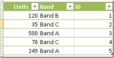
The formula works even if we have repeated ‘Band’ values.  In that case, I suggest adding an identity column to the table in order to break down the resulting value accordingly –

  Output:

This post has been featured on Excel’s MVP Bill Jelen “VLOOKUP Week” (March 25 – 31, 2012 ) which groups podcasts and blogs describing the use of this and other interesting Excel-related lookup functions and techniques. For more information, visit Microsoft’s Excel team blog @ http://tinyurl.com/c2aw89y , or directly access VLOOKUP’s week website @ http://vlookupweek.wordpress.com/

USERELATIONSHIP and direction of context propagation

My friend Hrvoje Piasevoli ( twitter ) pointed out to me recently that when using USERELATIONSHIP in a calculated column, the output was not the expected value based on the selected relationship.   I have used USERELATIONSHIP successfully in DAX measures a good number of times so I was surprised to hear the news.

In my effort to replicate the issue so I could better understand it, I used a calculated column on a BISM Tabular model based on the Adventure Works database.  The expression, on the FactInternetSales table, was as follows:

CALCULATE( VALUES(DimDate[DateKey] ) ,

USERELATIONSHIP( FactInternetSales[ShipDateKey], DimDate[DateKey] )

)

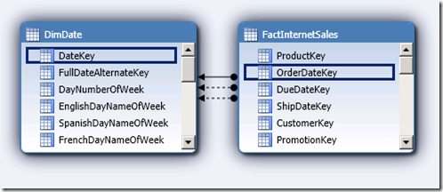
When using these tables in a Tabular model, the default ‘active’ relationship on this table is based on Order Date:

Clearly, the output I expected was the [DateKey] value associated with the current row through the relationship defined using the [ShipDateKey]. In other words, I expected the output to be the same as what the row showed for Ship Date.

Interestingly, the value I got back completely ignored the USERELATIONSHIP and was based on the active relationship using Order Date:

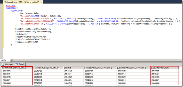
So is it that USERELATIONSHIPS are only supported on Measures and not Calculated Columns?  Not quite.  The problem is not with the type of DAX expression but with the direction of context propagation.  As an example, lets examine the following DAX query on the same Tabular model (click the image to expand it):

ADDCOLUMNS is the equivalent expression to adding a Calculated Column in the Grid pane of BISM Tabular or PowerPivot. And as you can see, neither of the expressions using USERELATIONSHIP returned the expected value.  The only expression that returned the correct Ship Date was the one using a calculated relationship based on FILTER, which did not leverage the model’s defined relationships.

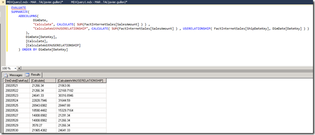
However, if we reverse the expression and evaluate it from the lookup table (DimDate), we get:

In other words, from the lookup table to the base table, USERELATIONSHIP works just fine.  The issue only emerges when invoking the function from the base table and making a call into the lookup table.

In DAX, context is automatically propagated from the lookup table to the base table.  In other words, when you assign filter context on a lookup table, only the corresponding base table rows are activated and taken into account when resolving the expression.  I described this on a prior blog entry related to Tabular relationships (Point # 2 here.)  Propagating context in the other direction does not happen automatically, and one must use functions like CALCULATE or RELATEDTABLE to generate this effect.

In this case, though, even using CALCULATE is not sufficient to propagate the context appropriately and one must use a calculated relationship.  In general terms, this should not be very problematic. However, the expression cannot benefit from the superior query performance delivered by leveraging the model’s defined relationships.

So in summary, USERELATIONSHIP can be used in both, Measures and Calculated Columns.  However – be mindful of the relationship direction as context will only respect USERELATIONSHIP when the filter is generated from the lookup table. Use a calculated relationship if you must place the filter on the base table.