Working with relationships in PowerPivot & SSAS BISM Tabular

Relationships in PowerPivot and SQL Server Analysis Services BISM Tabular can be a bit tricky.  It is easy to start with a few simple ones only to end up stuck at some point trying to figure out why table values are not rolling up across relationships as you would expect.

Particularly with PowerPivot,  it is easy to get the feeling you can just throw some tables are it, connect them and you should be ready to go.

Not so fast, though. There are specific rules to be followed when establishing valid relationships in PowerPivot and SSAS BISM Tabular. Understanding them is very important in order to get the most of these great analytical tools. Here is a list of the most important points to keep in mind:

1. Relationships must be based on a valid lookup.

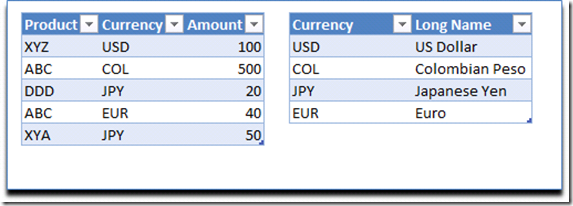
When you relate two tables, one must be the lookup for the other one. This is really another way of referring to a dimensional structure. For example:

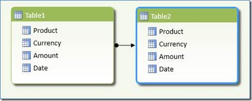
These two tables can be easily related in the model. PowerPivot will not complain at all, as the lookup table on the right contains unique entries for key column used to define the relationship (Currency).

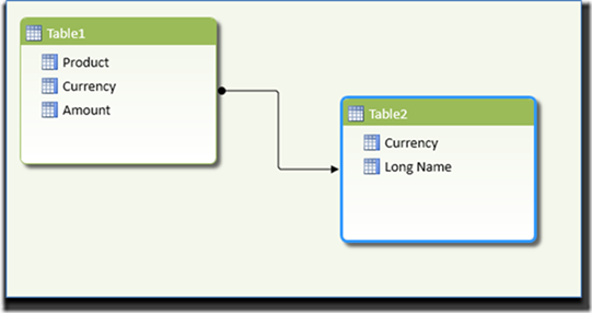
In the PowerPivot Window diagram, we can visualize this relationship as follows:

If you think about it this rule matches the way traditional UDM/OLAP cubes work: they also expect dimension tables to have unique key values. And this is really another way of saying: PowerPivot and BISM Tabular love star schemas. However, a star schema is not required and this technology opens the path to more flexible data modeling structures as cleverly pointed out by Marco Russo on his presentation on BISM Tabular data modeling: http://sqlbits.com/Sessions/event9/Vertipaq_vs_OLAP_Change_Your_Data_Modeling_Approach

2. Context is automatically propagated from the lookup table to the base table.

I have seen plenty of people getting stuck on this one, particularly when using PowerPivot for self service Business Intelligence.

Suppose you have the following tables:

As you can see, all currencies have a unique entry on each of the tables. So if you establish a relationship among them by using currency as the key, who is the lookup of who? PowerPivot will not complain when you create such a relationship.

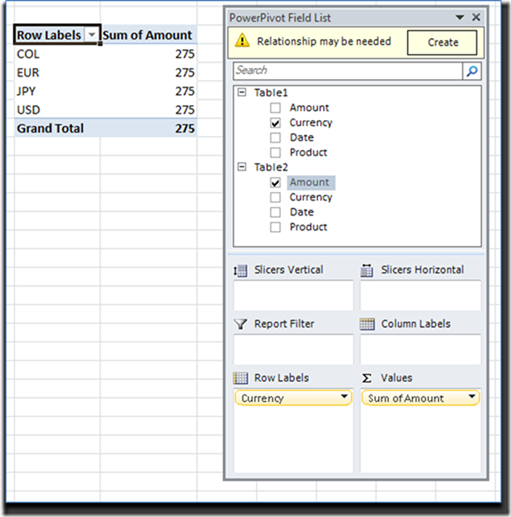
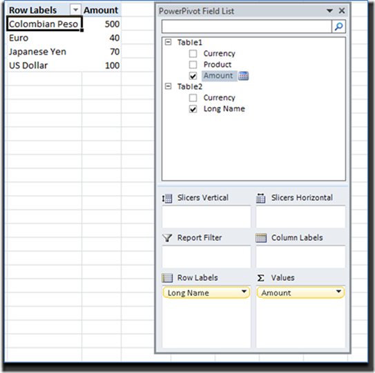
However, if we try to pivot the data, we will see the following:

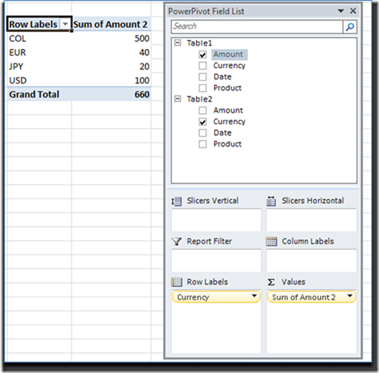
The results show numbers that are not being properly sliced when involving both tables. PowerPivot even complains by saying there is a missing relationship even though we have one! Notice in the field list that we selected the Currency from Table1 and Amount from Table2, so let’s try reversing this now and select the Currency from Table2 and Amount from Table1. We get the following:

This time the numbers are sliced appropriately! Why? Let’s examine the relationships again.

Table2 is the lookup table. As such, context is automatically propagated from it to the base table (Table1 in this case). This means that if I use Table1 as my categories or ‘dimension’ and Table2 as my metrics or ‘measures’ then relationships work fine without extra work on my side, and reports involving both tables will slice and dice as expected.

However, if I reverse this and use Table1 for my ‘measures’ and Table2 as for my categories (dimension) then context does not automatically propagate from one to the other one, which results in the pivot table giving the total amount for all currencies – and this is repeated for each currency in the row labels. In other words, it cannot grasp what the amount is for USD or for JPY or any other currency. It behaves in a similar way to a UDM cube when there is no specified dimension usage between a measure group and a dimension – it tries to evaluate context by using the [All] member if there is one.

In this model I have chosen to define Table2 as the lookup table but I could have defined it the other way, with Table1 being the lookup. As there are unique values on the key column, either relationship is possible.  However, context will still only automatically propagate in one way: from the lookup table to the base table.

You can force the context to propagate in reverse, by using DAX (see point #5 below).

3. Context can propagate many through many levels

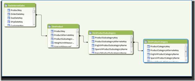
PowerPivot and BISM Tabular can handle snowflake schema relationships without a problem. Given the one-directional automatic context propagation described above, you can retrieve the value on one base table from a lookup table that is two or more levels away from it. For example:

On this snowflake schema, the table on the left contains the measures (Amount) and is the ‘base table’. The other three tables on the right have a descriptions for product, subcategory and category and they are all ‘lookup tables’.  In fact each table is a lookup to the next one (subcategory is a lookup to product, and category is a lookup to subcategory).

However, the Product table is the only one that has a direct relationship with the base table (FactInternetSales). And without us having to manipulate context, we can easily reach the “English Product Category Name”  from the base  table on the left all the way to the product category table all the way on the right, without a problem at all.  For this, we use the following DAX as a calculated column on the base table.

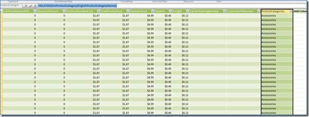
RELATED(DimProductCategory[EnglishProductCategoryName])

This is what the result looks like from the FactInternetSales table. The column highlighted was able to jump across two relationships, reaching a table three levels away:

These calculations are normally used to denormalize the model to – among other things – achieve a more user friendly experience as they browse the model from a client tool (Excel in the case of PowerPivot)

4. Relationships in the tabular model can be calculated.

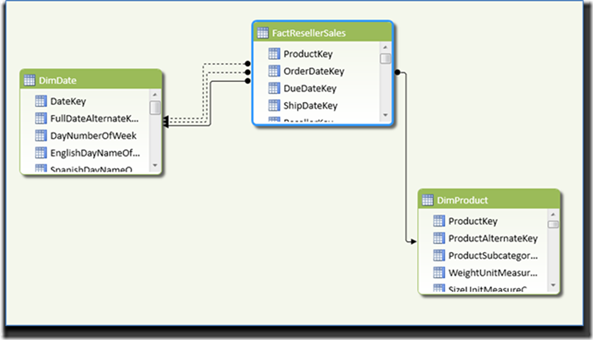
Unlike traditional OLAP/UDM cubes, relationships in PowerPivot and BISM Tabular can follow different paths at calculation runtime which can accommodate the equivalent of different versions of the data model based on calculation needs. For example, look at this data model diagram taken from a PowerPivot application:

As you can see there are three relationships between DimDate and FactResellerSales. This does not work exactly in the same way traditional SSAS role playing dimensions work; in PowerPivot and BISM Tabular, relationships can be active or inactive.

In a data model like the one above, a relationship path can be activated on the fly through the ‘UseRelationship()’ function:

CALCULATE( SUM( FactResellerSales[SalesAmount] ),

          USERELATIONSHIP(FactResellerSales[ShipDateKey], DimDate[DateKey])

)

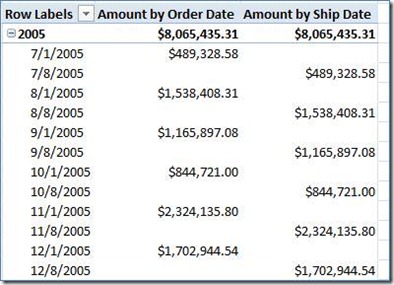
A relationship will be ‘active’ for the scope of execution of the calculation. By using this approach calculations that involve relationships can resolve using different paths in the same model, achieving results like this one:

The middle column uses the default relationship – so there is no need to invoke the UseRelationship() function here.  However,  the third column explicitly activates a different relationship path by using the DAX measure specified above.

Aside from this neat feature that gives lots of flexibility to the data model it is also possible to create pure calculated relationships. These do not rely on activating relationships already existing on the data model, but they literally generate the entire lookup operation as part of the formula evaluation.

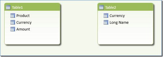
For example, If we use the same tables in point # 1, but delete the relationship from the data model we get:

Notice there are no relationships at all. However, we can still generate the following pivot table:

How is this possible? As you can see, the amount has been properly sliced based on the currency ‘long name’ attribute, which is only present in Table2. Clearly, this operation involves both tables. In order to generate a calculated relationship on the fly, we can define the following DAX expression:

IF(

HASONEVALUE(Table2[Currency]),

       CALCULATE( SUM( Table1[Amount_base] ),

                  FILTER(Table1, Table1[Currency] = VALUES(Table2[Currency]) )

                   )

    )

On it, the aggregate definition of SUM(Table1[Amount_base]) is modified by a filter context in which only the currency on Table1 that matches the current currency in context on Table2 will be used.

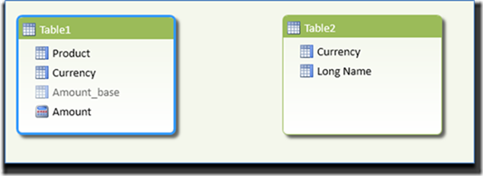
In addition to this, you perhaps noticed the aggregate function refers to an [Amount _base] column that did not exist on the original data model. I did this to keep the model user-friendly, by replacing the original measure with a new measure defined by the DAX calculation we defined above. In order to do this, I had to rename the original measure as two measures cannot have the same name. I called that original measure [Amount_base] and configured it to be hidden, which resulted in the following in-memory data model:

The [Amount] measure was defined as a DAX measure whereas the [amount_base] now appears grayed out as client tools won’t be able to see it anymore. This avoids potential user confusion of having to look at two fields with similar names.

5. DAX calculations can modify the way context is propagated by default.

As you may recall from point # 2, context automatically propagates in one direction – from the lookup table to the base table. However, this can be modified by the use of DAX.

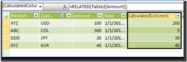
Let’s take the same example used on point # 2. By using the RELATED() function, we are able to reach out to a lookup table and grab a value based on the current row context. For example, if we are looking at base table ‘Table1’ and use the RELATED() function in a calculated column, we are able to fetch the related Amount value on Table2 for the currency in current context on Table1.

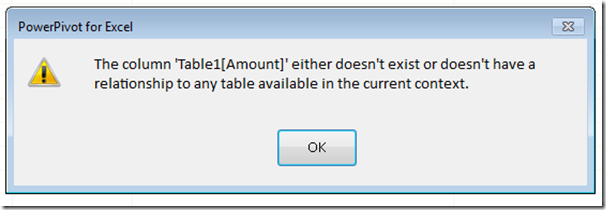
However, if we try to do the same operation from the lookup table, Table2, we get an error:

The error, when expanded, shows this:

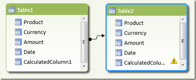
Remember that in our example each table had unique currency values so any table could have been defined as the lookup. And this is the same exact behavior we got with the pivot tables on point #2: context will automatically propagate only one way- from the lookup table to the base table. In this case, I am unable to reach Table1 from Table2, as Table1 is not defined as the lookup table in the relationship.

As we saw before, this is not the case when trying to get the related values on Table2 (the lookup) from Table1 (the base).  Things here work as expected and without errors. Both attempts are reflected in the data model diagram above in which the last column on Table2 has a warning message next to it signaling it wasn’t able to successfully resolve the computation.

We can override this behavior by using the CALCULATE() function. Replacing the bad calculation in Table2 with the calculation below will allow us to propagate context in the other direction and fetch the right values from Table1 to the current currency in context in Table2, even if Table2 is still defined as the lookup table:

CALCULATE(SUM(Table1[Amount]))

Why is this? Because CALCULATE() automatically turns row context into filter context. What this means is that for the currency in context – as the formula evaluates row by row – is able to reach out to the other table following the relationship and select the subset of rows on that table that pertain to this currency. In our example  there is only one matching row on the other side of the relationship but even if we were to have many rows on the other side we would be able to aggregate them properly (we are specifying the use of the aggregate SUM() function as part of the formula expression. Clearly, we can also use other aggregate functions like MIN(), MAX(), etc.).

Another way we could have done this is by using RELATEDTABLE() as internally this function can also propagate context on the reverse:

SUMX(RELATEDTABLE(Table1), Table1[Amount])

I would recommend sticking with the approach using CALCULATE() if possible as not only is faster than SUMX() but in many cases it is easier to troubleshoot.

You may wonder: why use calculated relationships when one could stick to regular relationships? The reason is that there are some business problems that require the use of flexible data models that may not be able to leverage regular relationships, yet with the use of calculated relationships it is possible to find a working – and elegant – solution. A great example of this is the use of calculated relationships to define banding, as explained in this great article by Alberto Ferrari: http://sqlblog.com/blogs/alberto_ferrari/archive/2010/10/12/banding-with-powerpivot.aspx

Hopefully this post will assist with clarifying many of the confusions out there regarding how relationships work. Once you become aware of the principles behind valid relationships and their impact in calculation context it will be easier to generate insightful PowerPivot reports or versatile BISM Tabular models.